0. Set up

Code

# cleaning
library(tidyverse)

# visualization
theme_set(theme_classic() +
            theme(panel.grid = element_blank(),
                  axis.text = element_text(size = 18),
                  axis.title = element_text(size = 18),
                  text = element_text(family = "Lato")))
library(patchwork)
library(ggeffects)
library(flextable)
library(modelsummary)
library(gtsummary)
library(readxl)
library(here)
library(janitor)

# analysis
library(car)
library(performance)
library(broom)

1. Math

a. Residuals

Residuals are the difference between the actual observed value ($y_i$) and the model prediction ($\hat{y}$) at some value of $x$.

\[ residual = y_i - \hat{y} \]

Ordinary least squares minimizes the sum of squares of the residuals.

b. Model equations

OLS gives you an equation for a line.

$$ \[\begin{align} y &= b + mx \\ y &= \beta_0 + \beta_1x + \epsilon \\ \end{align}\] $$ $\beta$ terms (“betas”) are often referred to as “model coefficients”.

c. Mathematical hypothesis

Statistically, the hypotheses are:

H_0_: the predictor variable does not predict the response
H_A_: the predictor variable does predict the response

Mathematically, you might express that as:

\[ H_0: \beta_1 = 0 \\ H_A: \beta_1 \neq 0 \]

d. R2

\[ \begin{align} R^2 &= 1 - \frac{\sum_{i = 1}^{n}(y_i - \hat{y})^2}{\sum_{i = 1}^{n}(y_i - \bar{y})^2} \\ &= 1 - \frac{SS_{residuals}}{SS_{total}} \end{align} \]

e. Pearson’s correlation

formula for Pearson’s correlation

\[ r = \frac{\sum(x_i - \bar{x})(y_i - \bar{y})}{\sqrt{\sum(x_i-\bar{x})^2}\sqrt{\sum(y_i - \bar{y})^2}} \]

test statistic for pearson correlation

\[ \begin{align} t &= \frac{r\sqrt{n - 2}}{\sqrt{1-r^2}} \\ df &= n -2 \end{align} \]

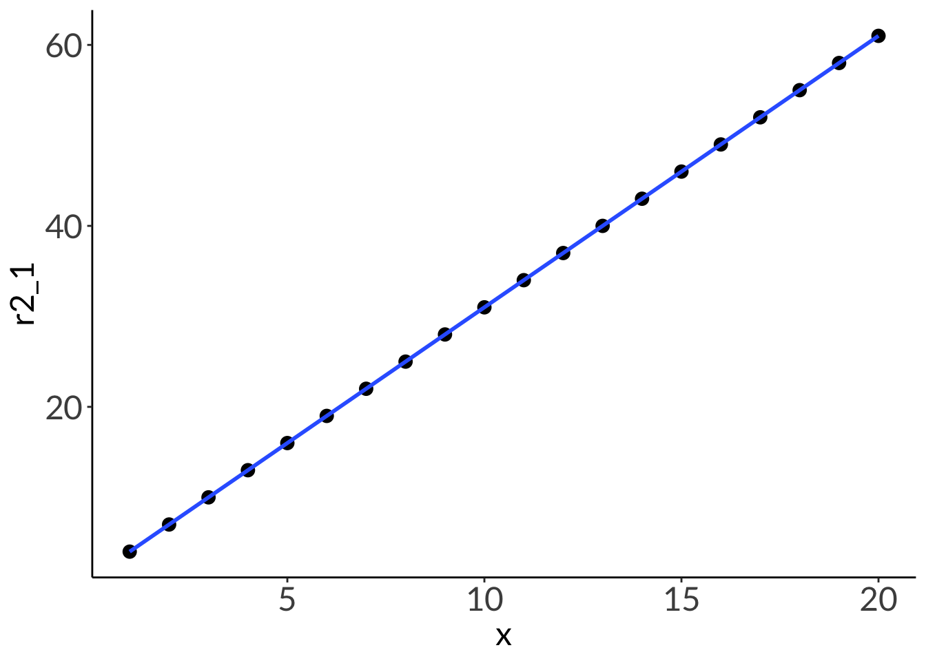
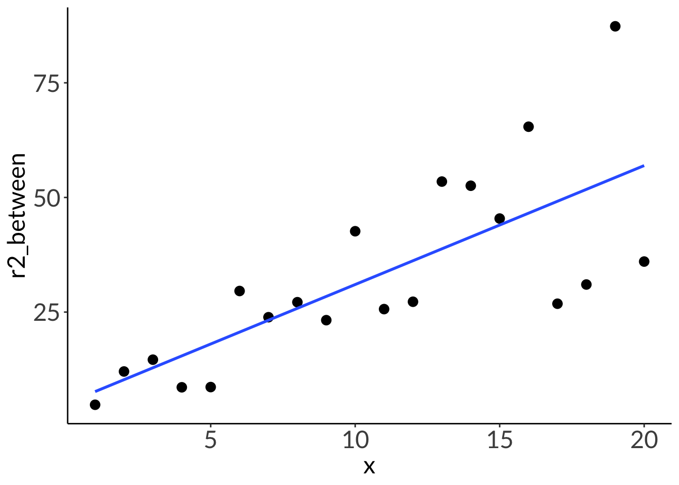
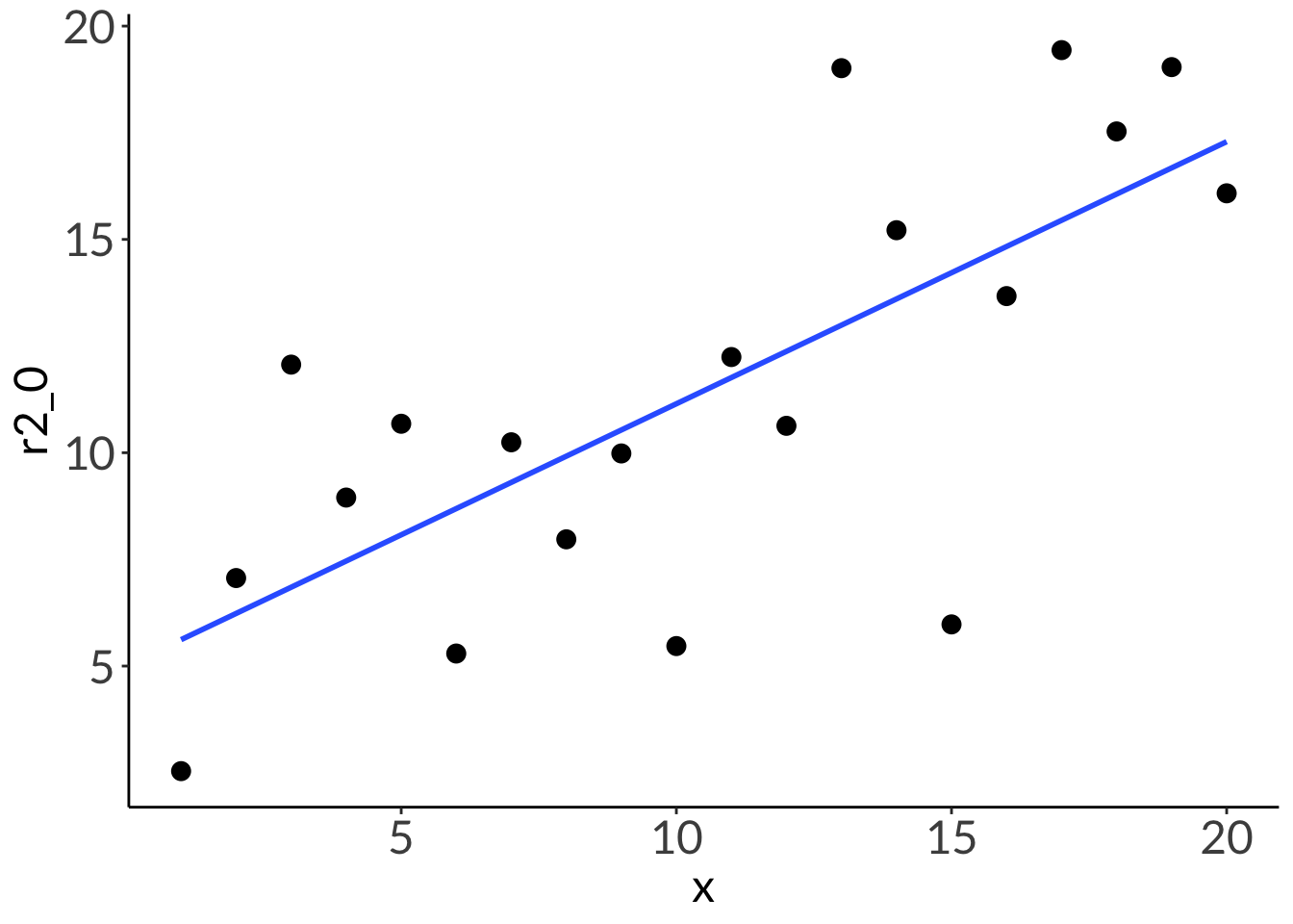
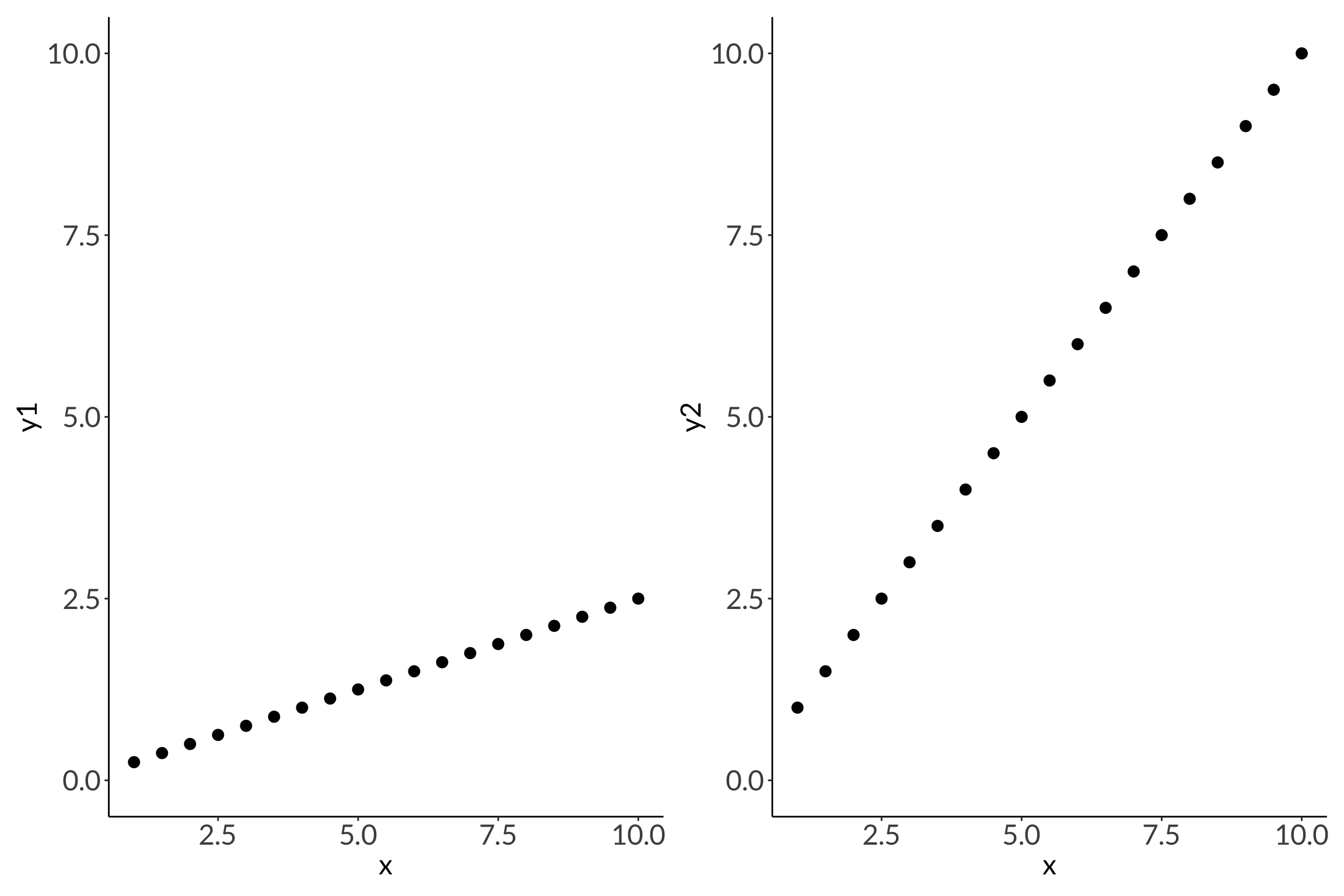
2. R2

Code

df <- tibble(
  x = seq(from = 1, to = 20, by = 1),
  r2_1 = 3*x + 1,
  r2_between = runif(n = 20, min = 1, max = 5)*x + runif(n = 20, min = 1, max = 5),
  r2_0 = runif(n = 20, min = 1, max = 20)
)

lm(r2_1 ~ x, data = df) |> 
  summary()


Call:
lm(formula = r2_1 ~ x, data = df)

Residuals:
       Min         1Q     Median         3Q        Max 
-3.676e-15 -1.312e-15 -5.240e-17  8.432e-16  7.220e-15 

Coefficients:
             Estimate Std. Error   t value Pr(>|t|)    
(Intercept) 1.000e+00  1.142e-15 8.757e+14   <2e-16 ***
x           3.000e+00  9.532e-17 3.147e+16   <2e-16 ***
---
Signif. codes:  0 '***' 0.001 '**' 0.01 '*' 0.05 '.' 0.1 ' ' 1

Residual standard error: 2.458e-15 on 18 degrees of freedom
Multiple R-squared:      1, Adjusted R-squared:      1 
F-statistic: 9.905e+32 on 1 and 18 DF,  p-value: < 2.2e-16

Code

ggplot(df,
       aes(x = x,
           y = r2_1)) +
  geom_point(size = 3) +
  geom_smooth(method = "lm")

Code

lm(r2_between ~ x, data = df) |> 
  summary()


Call:
lm(formula = r2_between ~ x, data = df)

Residuals:
    Min      1Q  Median      3Q     Max 
-22.344  -8.201   0.994   9.517  32.971 

Coefficients:
            Estimate Std. Error t value Pr(>|t|)    
(Intercept)   5.0684     6.6511   0.762  0.45591    
x             2.5942     0.5552   4.672  0.00019 ***
---
Signif. codes:  0 '***' 0.001 '**' 0.01 '*' 0.05 '.' 0.1 ' ' 1

Residual standard error: 14.32 on 18 degrees of freedom
Multiple R-squared:  0.5481,    Adjusted R-squared:  0.523 
F-statistic: 21.83 on 1 and 18 DF,  p-value: 0.0001896

Code

ggplot(df,
       aes(x = x,
           y = r2_between)) +
  geom_point(size = 3) +
  geom_smooth(method = "lm",
              se = FALSE)

Code

lm(r2_0 ~ x, data = df) |> 
  summary()


Call:
lm(formula = r2_0 ~ x, data = df)

Residuals:
    Min      1Q  Median      3Q     Max 
-8.2426 -1.7958  0.6555  1.7988  6.0232 

Coefficients:
            Estimate Std. Error t value Pr(>|t|)    
(Intercept)   5.0045     1.6667   3.003 0.007641 ** 
x             0.6143     0.1391   4.415 0.000334 ***
---
Signif. codes:  0 '***' 0.001 '**' 0.01 '*' 0.05 '.' 0.1 ' ' 1

Residual standard error: 3.588 on 18 degrees of freedom
Multiple R-squared:  0.5199,    Adjusted R-squared:  0.4932 
F-statistic: 19.49 on 1 and 18 DF,  p-value: 0.0003342

Code

ggplot(df,
       aes(x = x,
           y = r2_0)) +
  geom_point(size = 3) +
  geom_smooth(method = "lm",
              se = FALSE)

3. Red abalone example

This example is inspired in by Hamilton et al. 2022.

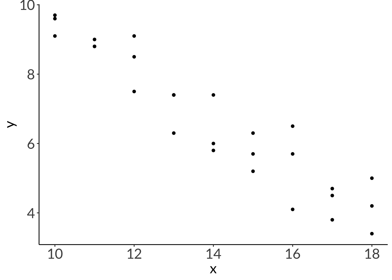
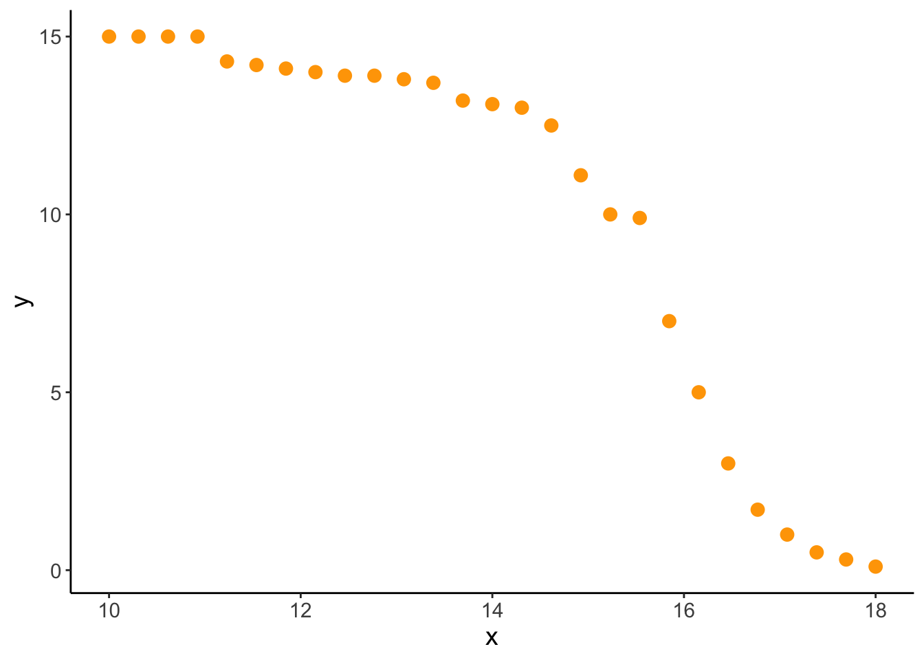
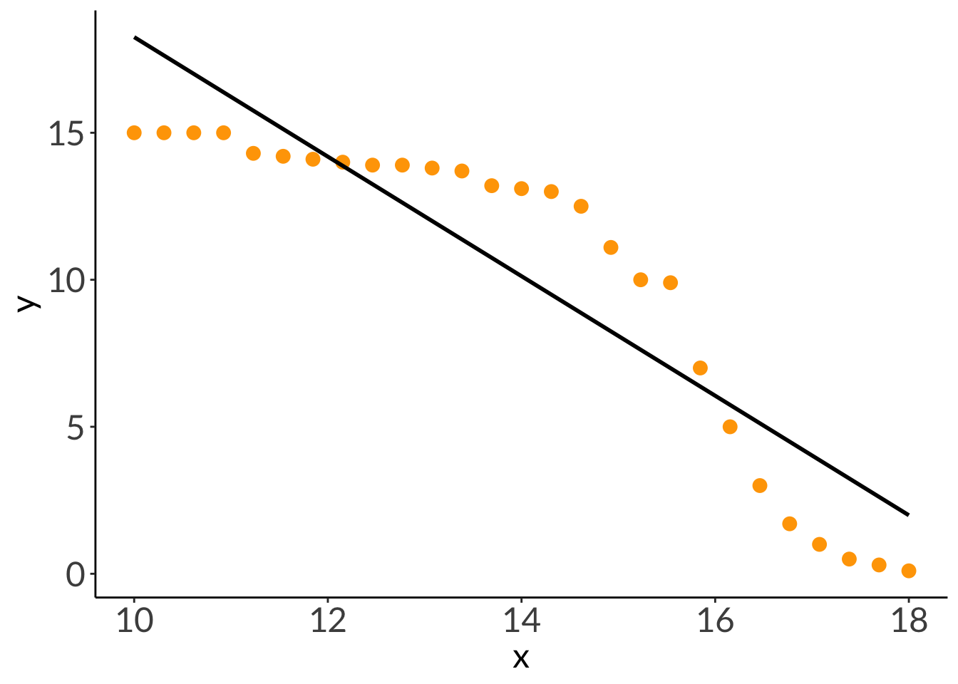
We work with the linear model using the real data in class, but it’s hard to see the difference in diagnostic plots between a “good” vs “bad” linear model with that data set.

This is the fake data generated to compare different diagnostic plots.

a. generating the data

Code

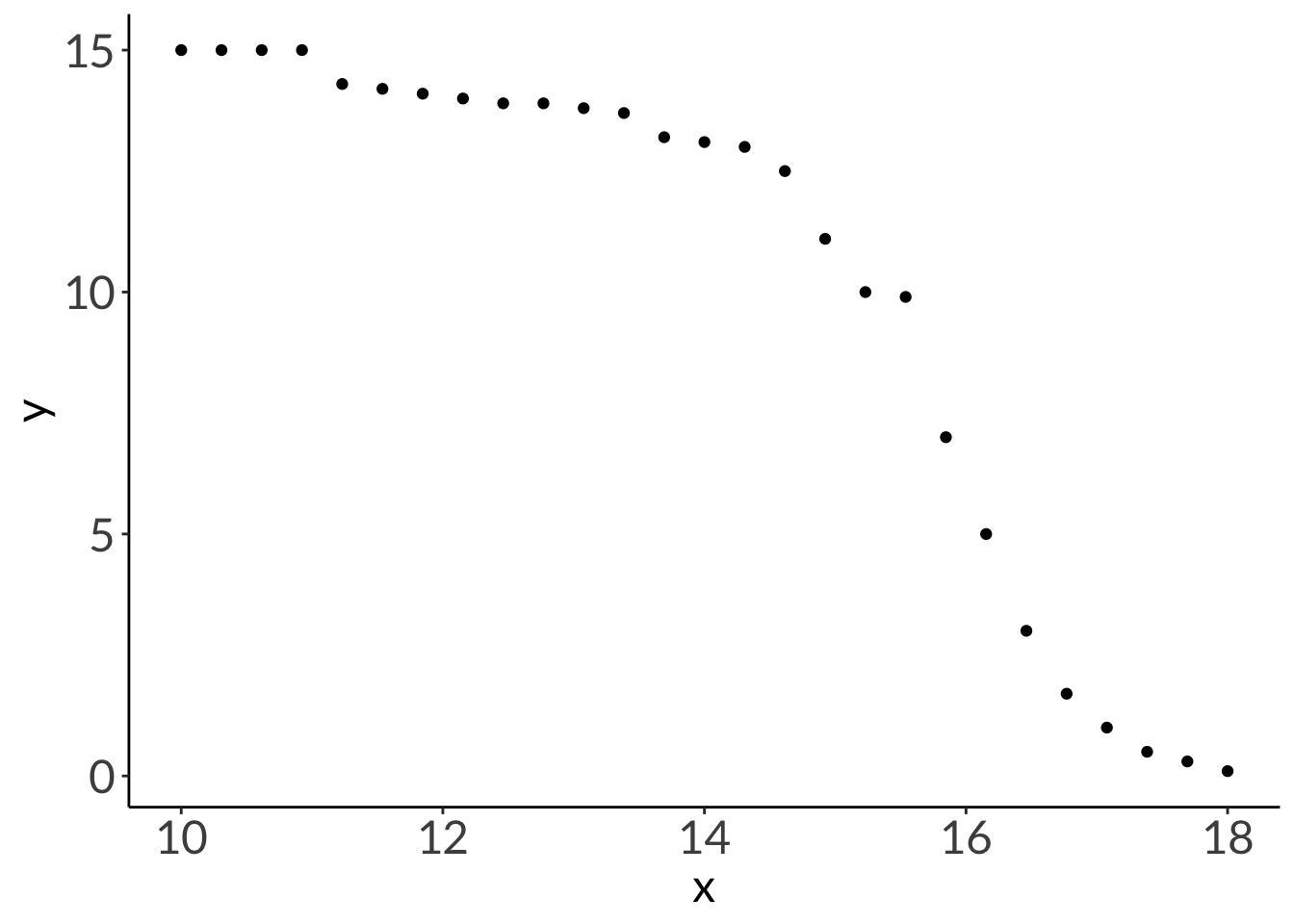
set.seed(666)
abalone <- tibble(
  temperature = seq(from = 10, to = 18, by = 1),
  growth1 = runif(length(temperature), min = -0.7, max = -0.63)*temperature + runif(length(temperature), min = 15, max = 17),
  growth2 = runif(length(temperature), min = -0.7, max = -0.63)*temperature + runif(length(temperature), min = 15, max = 17),
  growth3 = runif(length(temperature), min = -0.7, max = -0.63)*temperature + runif(length(temperature), min = 15, max = 17)
) |> 
  pivot_longer(cols = growth1:growth3,
               names_to = "rep",
               values_to = "growth") |> 
  mutate(growth = round(growth, digits = 1)) |> 
  select(temperature, growth) |> 
  rename(x = temperature,
         y = growth)

# look at your data:
head(abalone, 10)

# A tibble: 10 × 2
       x     y
   <dbl> <dbl>
 1    10   9.1
 2    10   9.6
 3    10   9.7
 4    11   9  
 5    11   8.8
 6    11   8.8
 7    12   7.5
 8    12   9.1
 9    12   8.5
10    13   6.3

Code

ggplot(data = abalone,
       aes(x = x,
           y = y)) +
  geom_point()

Seems like there is a linear relationship between temperature and abalone growth. As temperature increases, abalone growth decreases.

b. fitting a model

Code

abalone_model <- lm(
  y ~ x,
  data = abalone
)

# just checking DHARMa residuals just in case
DHARMa::simulateResiduals(abalone_model, plot = TRUE)

Object of Class DHARMa with simulated residuals based on 250 simulations with refit = FALSE . See ?DHARMa::simulateResiduals for help. 
 
Scaled residual values: 0.328 0.604 0.656 0.62 0.548 0.472 0.228 0.976 0.716 0.052 0.496 0.528 0.128 0.132 0.92 0.352 0.684 0.152 0.98 0.764 ...

Code

# base R residuals
par(mfrow = c(2, 2))
plot(abalone_model)

c. looking at model coefficients

Code

summary(abalone_model)


Call:
lm(formula = y ~ x, data = abalone)

Residuals:
     Min       1Q   Median       3Q      Max 
-1.15370 -0.50093  0.06019  0.34491  1.24630 

Coefficients:
            Estimate Std. Error t value Pr(>|t|)    
(Intercept) 16.40926    0.69633   23.57  < 2e-16 ***
x           -0.69722    0.04891  -14.25 1.65e-13 ***
---
Signif. codes:  0 '***' 0.001 '**' 0.01 '*' 0.05 '.' 0.1 ' ' 1

Residual standard error: 0.6562 on 25 degrees of freedom
Multiple R-squared:  0.8904,    Adjusted R-squared:  0.8861 
F-statistic: 203.2 on 1 and 25 DF,  p-value: 1.65e-13

Code

# common way of representing model summaries
# from flextable package
flextable::as_flextable(abalone_model)

	Estimate	Standard Error	t value	Pr(>\|t\|)
(Intercept)	16.409	0.696	23.565	0.0000	***
x	-0.697	0.049	-14.254	0.0000	***
Signif. codes: 0 <= '*' < 0.001 < '' < 0.01 < '*' < 0.05

Residual standard error: 0.6562 on 25 degrees of freedom
Multiple R-squared: 0.8904, Adjusted R-squared: 0.8861
F-statistic: 203.2 on 25 and 1 DF, p-value: 0.0000

Code

# better table
flextable::as_flextable(abalone_model) |> 
  set_formatter(values = list("p.value" = function(x){ # special function to represent p < 0.001
    z <- scales::label_pvalue()(x)
    z[!is.finite(x)] <- ""
    z
  }))

	Estimate	Standard Error	t value	Pr(>\|t\|)
(Intercept)	16.409	0.696	23.565	<0.001	***
x	-0.697	0.049	-14.254	<0.001	***
Signif. codes: 0 <= '*' < 0.001 < '' < 0.01 < '*' < 0.05

Residual standard error: 0.6562 on 25 degrees of freedom
Multiple R-squared: 0.8904, Adjusted R-squared: 0.8861
F-statistic: 203.2 on 25 and 1 DF, p-value: 0.0000

Code

# somewhat more customizable way
# from modelsummary package
modelsummary(abalone_model)

	(1)
(Intercept)	16.409
	(0.696)
x	-0.697
	(0.049)
Num.Obs.	27
R2	0.890
R2 Adj.	0.886
AIC	57.8
BIC	61.7
Log.Lik.	-25.899
F	203.189
RMSE	0.63

Code

# better table
modelsummary(list("Abalone model" = abalone_model), # naming the model
             fmt = 2, # rounding digits to 2 decimal places
             estimate = "{estimate} [{conf.low}, {conf.high}] ({p.value})", # customizing appearance
             statistic = NULL, # not displaying standard error
             gof_omit = 'DF|AIC|BIC|Log.Lik.|RMSE') # taking out some extraneous info

	Abalone model
(Intercept)	16.41 [14.98, 17.84] (<0.01)
x	-0.70 [-0.80, -0.60] (<0.01)
Num.Obs.	27
R2	0.890
R2 Adj.	0.886
F	203.189

Code

# using gtsummary package
tbl_regression(abalone_model,
               intercept = TRUE)

Characteristic	Beta	95% CI	p-value
(Intercept)	16	15, 18	<0.001
x	-0.70	-0.80, -0.60	<0.001
Abbreviation: CI = Confidence Interval

Code

# more customizing
tbl_regression(abalone_model, # model object
               intercept = TRUE) |> # show the intercept
  as_flex_table() # turn it into a flextable (easier to save)

Characteristic	Beta	95% CI	p-value
(Intercept)	16	15, 18	<0.001
x	-0.70	-0.80, -0.60	<0.001
Abbreviation: CI = Confidence Interval

Code

anova(abalone_model)

Analysis of Variance Table

Response: y
          Df Sum Sq Mean Sq F value   Pr(>F)    
x          1 87.501  87.501  203.19 1.65e-13 ***
Residuals 25 10.766   0.431                     
---
Signif. codes:  0 '***' 0.001 '**' 0.01 '*' 0.05 '.' 0.1 ' ' 1

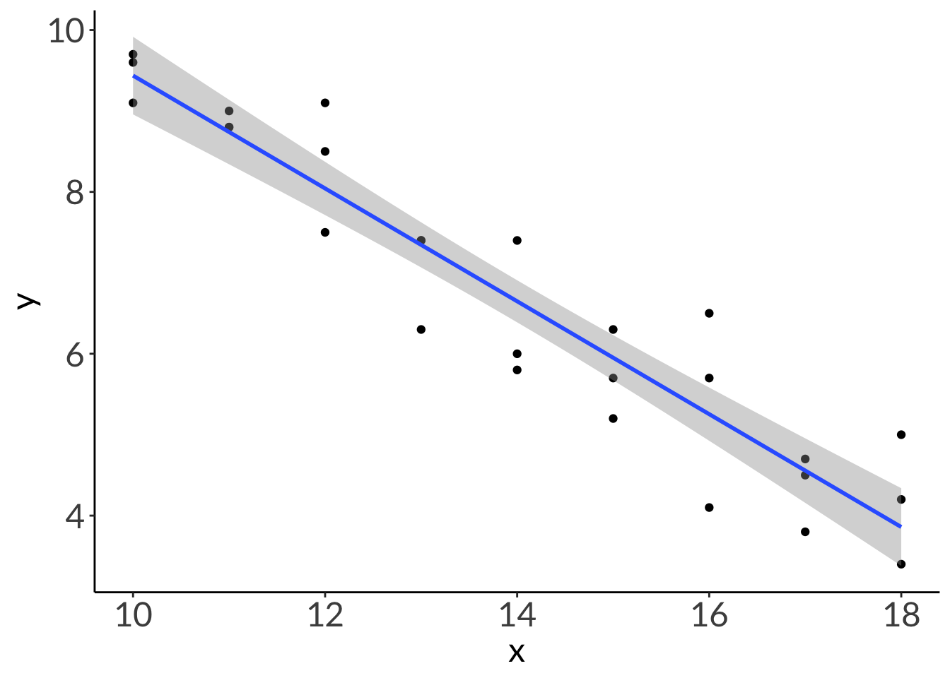
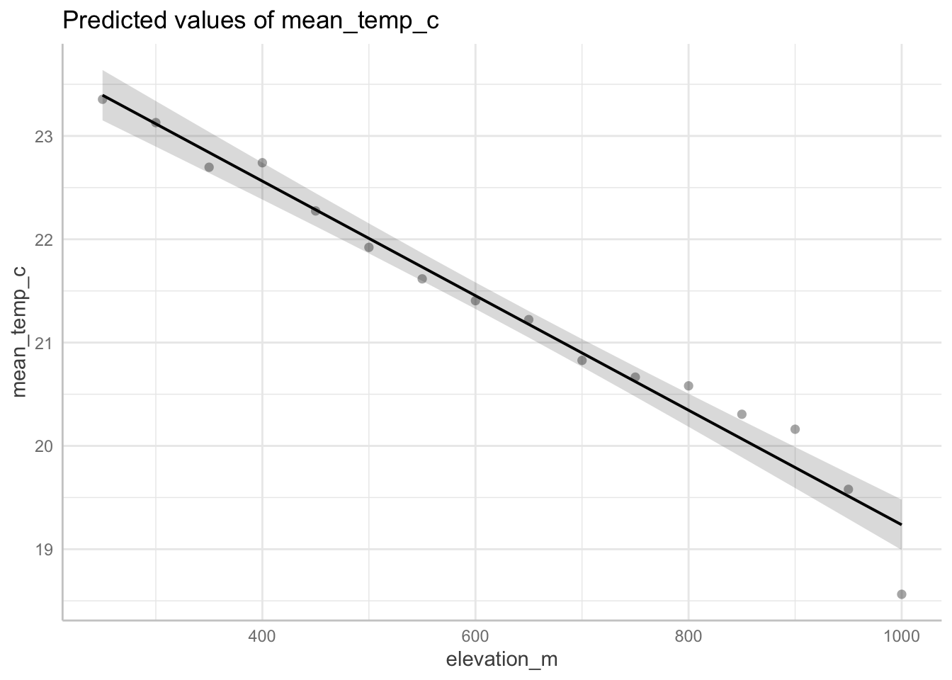
d. visualizing the model

Code

model_preds <- ggpredict(
  abalone_model,
  terms = "x"
)

# look at the output:
model_preds

# Predicted values of y

 x | Predicted |     95% CI
---------------------------
10 |      9.44 | 8.96, 9.92
11 |      8.74 | 8.34, 9.14
12 |      8.04 | 7.71, 8.37
13 |      7.35 | 7.07, 7.62
14 |      6.65 | 6.39, 6.91
15 |      5.95 | 5.67, 6.23
16 |      5.25 | 4.92, 5.58
18 |      3.86 | 3.38, 4.34

Code

ggpredict(abalone_model, 
          terms = "x[18]")

# Predicted values of y

 x | Predicted |     95% CI
---------------------------
18 |      3.86 | 3.38, 4.34

Code

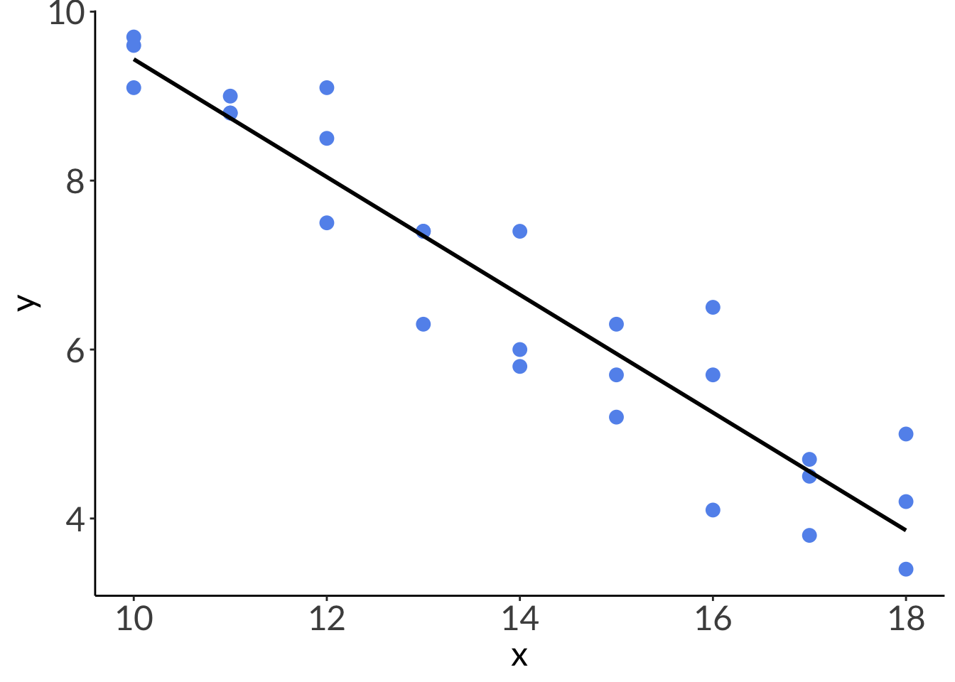
# plotting without 95% CI
ggplot(abalone, # using the actual data
       aes(x = x, # x-axis
           y = y)) + # y-axis
  geom_point(color = "cornflowerblue", # each point is an individual abalone
             size = 3) +
  
  # model prediction: actual model line
  geom_line(data = model_preds, # model prediction table
            aes(x = x, # x-axis
                y = predicted), # y-axis
            linewidth = 1)  # line width

Code

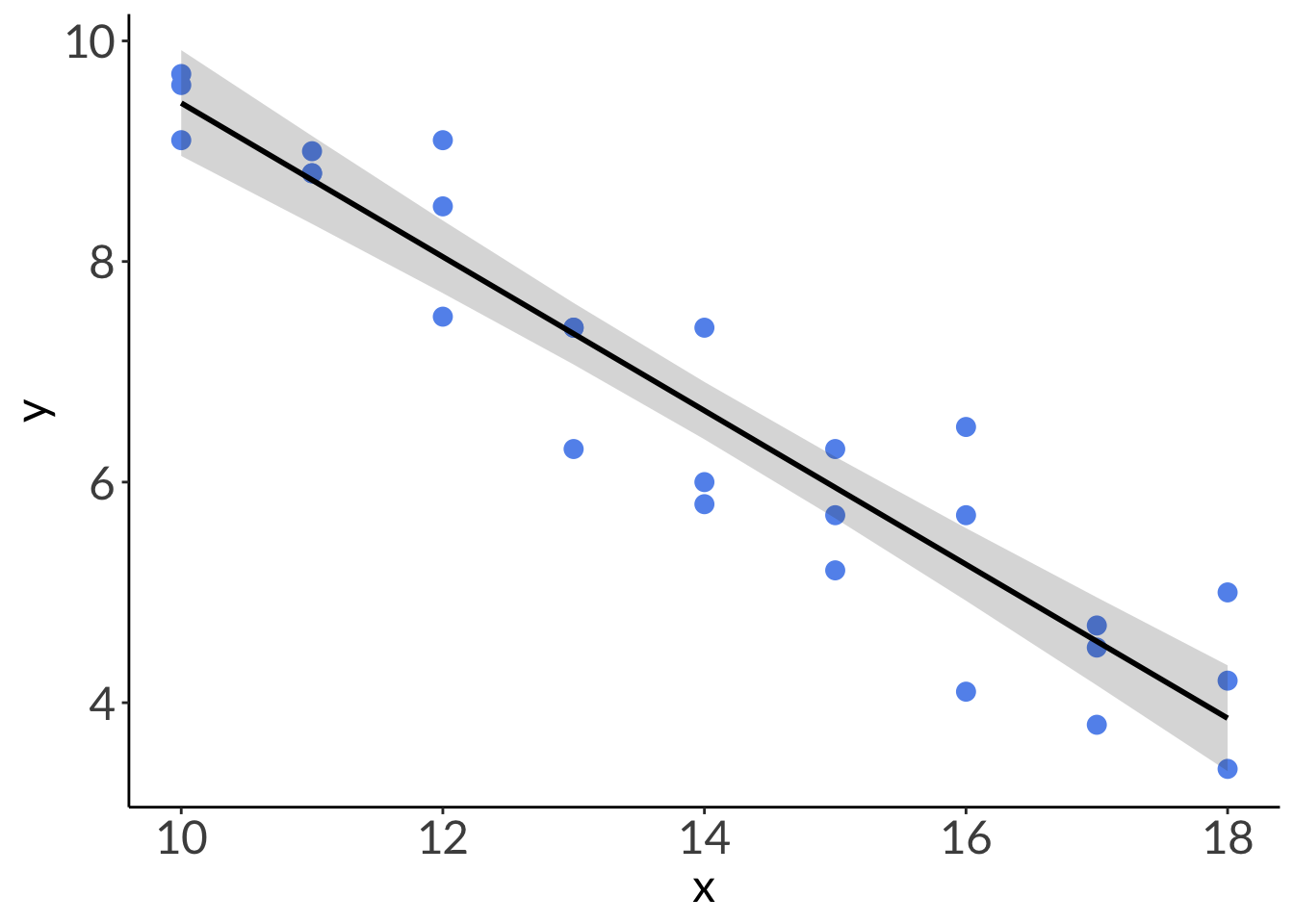
# plotting
ggplot(abalone, # using the actual data
       aes(x = x, # x-axis
           y = y)) + # y-axis
  
  # plot the data first
  # each point is an individual abalone
  geom_point(color = "cornflowerblue",
             size = 3) + 
  
  # model prediction: 95% CI
  geom_ribbon(data = model_preds, # model prediction table
              aes(x = x, # x-axis
                  y = predicted, # y-axis
                  ymin = conf.low, # lower bound of 95% CI
                  ymax = conf.high), # upper bound of 95% CI
              alpha = 0.2) + # transparency) 
  
  # model prediction: actual model line
  geom_line(data = model_preds, # model prediction table
            aes(x = x, # x-axis
                y = predicted), # y-axis
            linewidth = 1) # line width

Code

# compare with:
ggplot(abalone,
       aes(x = x,
           y = y)) +
  geom_point() +
  geom_smooth(method = "lm")

e. outliers

Code

abalone |> 
  mutate(outlier = ifelse(row_number() %in% c(19, 21, 27), "yes", "no")) |> 
  ggplot(aes(x = x,
             y = y)) +
  geom_point(aes(color = outlier), 
             size = 3) + 
  geom_line(data = model_preds,
            aes(x = x,
                y = predicted),
            linewidth = 1) +
  scale_color_manual(values = c("yes" = "red", "no" = "cornflowerblue")) +
  theme(legend.position = "none")

Code

# new abalone data frame
abalone2 <- abalone |> 
  slice(-c(19, 21, 27))

abalone_model2 <- lm(y ~ x,
                    data = abalone2)

summary(abalone_model2)


Call:
lm(formula = y ~ x, data = abalone2)

Residuals:
     Min       1Q   Median       3Q      Max 
-1.01641 -0.44359  0.08359  0.34163  1.05272 

Coefficients:
            Estimate Std. Error t value Pr(>|t|)    
(Intercept) 16.81772    0.60270   27.90  < 2e-16 ***
x           -0.73087    0.04336  -16.85 4.61e-14 ***
---
Signif. codes:  0 '***' 0.001 '**' 0.01 '*' 0.05 '.' 0.1 ' ' 1

Residual standard error: 0.537 on 22 degrees of freedom
Multiple R-squared:  0.9281,    Adjusted R-squared:  0.9249 
F-statistic: 284.1 on 1 and 22 DF,  p-value: 4.606e-14

Code

model_preds2 <- ggpredict(abalone_model2, terms = "x")

ggplot(data = abalone2,
       aes(x = x,
           y = y)) +
  geom_point(color = "cornflowerblue",
             size = 3) +
  geom_line(data = model_preds2,
            aes(x = x,
                y = predicted), 
            linewidth = 1)

f. actual data

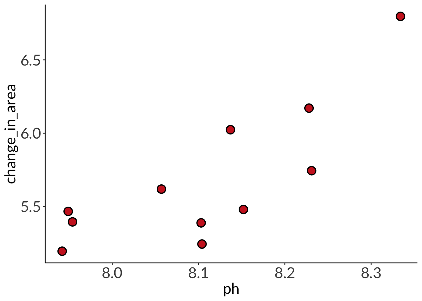
Data from: Hamilton et al. 2022. Aquaculture. “Integrated multi-trophic aquaculture mitigates the effects of ocean acidification: Seaweeds raise system pH and improve growth of juvenile abalone.”

Thank you to Scott for being willing to share this data!

Code

abalone <- read_xlsx(here("data", "Abalone IMTA_growth and pH.xlsx")) |> 
  clean_names()

# creating clean dataset
abalone_clean <- abalone |> # start with abalone object
  # select columns of interest
  select(mean_p_h, change_in_area_mm2_d_1_25, recirculation_treatment) |> 
  # rename columns
  rename(ph = mean_p_h, 
         change_in_area = change_in_area_mm2_d_1_25,
         recirculation = recirculation_treatment) |> 
  # recod recirculation
  mutate(recirculation = case_when(
    recirculation == 0 ~ "0% recirculation",
    recirculation == 0.3 ~ "30% recirculation",
    recirculation == 0.65 ~ "65% recirculation"
  ))

# base layer: ggplot
ggplot(data = abalone_clean,
       aes(x = ph,
           y = change_in_area)) +
  # first layer: points representing abalones
  geom_point(size = 4,
             stroke = 1,
             fill = "firebrick3",
             shape = 21)

Code

abalone_clean |> 
  select(ph, change_in_area) |> 
  slice_sample(n = 5)

# A tibble: 5 × 2
     ph change_in_area
  <dbl>          <dbl>
1  7.95           5.40
2  8.23           5.74
3  8.15           5.48
4  8.14           6.02
5  7.95           5.47

Code

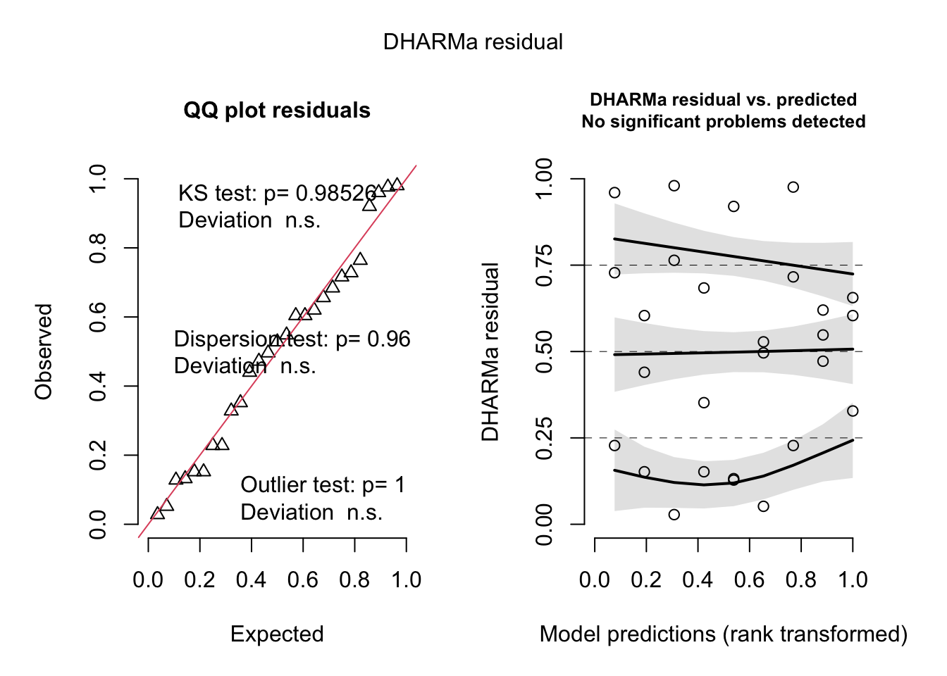
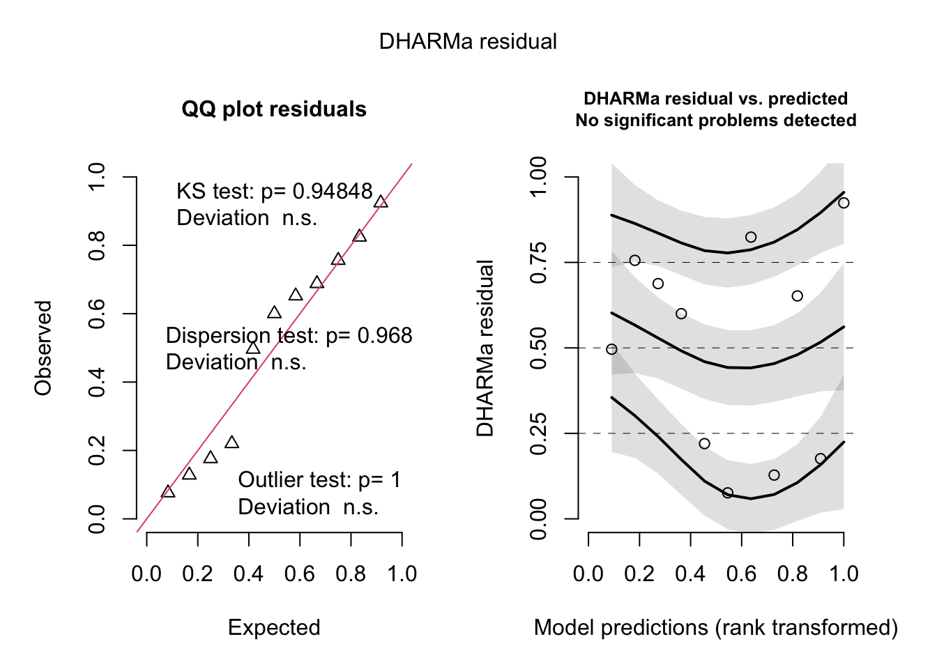
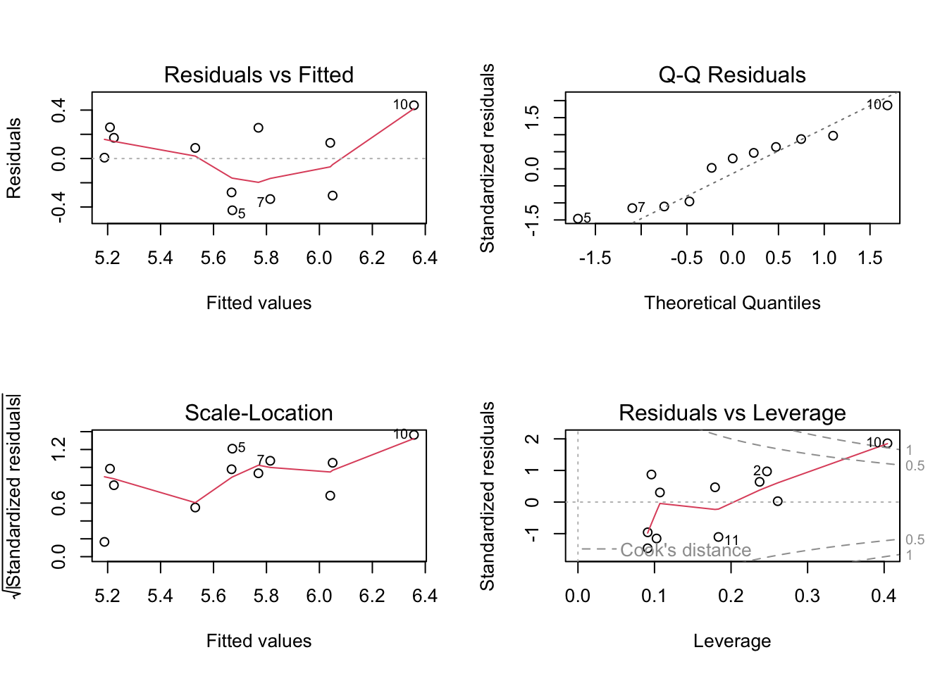
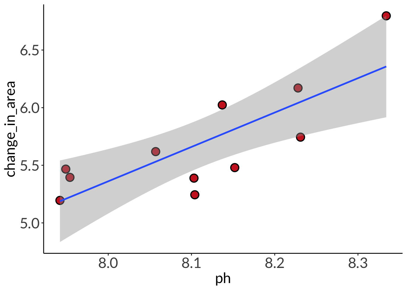
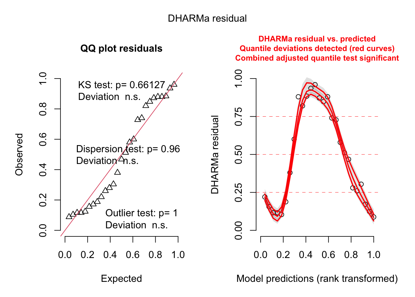
abalone_model <- lm(
  change_in_area ~ ph,  # formula: change in area as a function of pH
  data = abalone_clean  # data frame: abalone_clean
)

DHARMa::simulateResiduals(abalone_model) |> 
  plot()

Code

par(mfrow = c(2, 2))   # creating a 2x2 grid
plot(abalone_model)    # plot diagnostic plots

Code

# more information about the model
summary(abalone_model)


Call:
lm(formula = change_in_area ~ ph, data = abalone_clean)

Residuals:
     Min       1Q   Median       3Q      Max 
-0.42714 -0.29282  0.08769  0.21258  0.43965 

Coefficients:
            Estimate Std. Error t value Pr(>|t|)   
(Intercept) -18.5010     6.1601  -3.003  0.01488 * 
ph            2.9827     0.7596   3.926  0.00348 **
---
Signif. codes:  0 '***' 0.001 '**' 0.01 '*' 0.05 '.' 0.1 ' ' 1

Residual standard error: 0.3063 on 9 degrees of freedom
  (1 observation deleted due to missingness)
Multiple R-squared:  0.6314,    Adjusted R-squared:  0.5905 
F-statistic: 15.42 on 1 and 9 DF,  p-value: 0.003477

Code

# creating a new object called abalone_preds
abalone_preds <- ggpredict(
  abalone_model,      # model object
  terms = "ph"        # predictor (in quotation marks)
)

# display the predictions
abalone_preds

# Predicted values of change_in_area

  ph | Predicted |     95% CI
-----------------------------
7.94 |      5.19 | 4.83, 5.54
7.95 |      5.21 | 4.86, 5.55
8.06 |      5.53 | 5.30, 5.76
8.10 |      5.67 | 5.46, 5.88
8.10 |      5.67 | 5.46, 5.88
8.14 |      5.77 | 5.55, 5.98
8.15 |      5.81 | 5.59, 6.04
8.33 |      6.36 | 5.92, 6.80

Code

# find predicted growth at ph = 7.9
ggpredict(
  abalone_model,
  terms = "ph[7.9]"
)

# Predicted values of change_in_area

  ph | Predicted |     95% CI
-----------------------------
7.90 |      5.06 | 4.65, 5.48

Code

# find predicted growth at ph = 7.9
ggpredict(
  abalone_model,
  terms = "ph[8.23]"
)

# Predicted values of change_in_area

  ph | Predicted |     95% CI
-----------------------------
8.23 |      6.05 | 5.75, 6.34

Code

# find predicted growth at ph = 8
ggpredict(
  abalone_model,
  terms = "ph[8]"
)

# Predicted values of change_in_area

ph | Predicted |     95% CI
---------------------------
 8 |      5.36 | 5.08, 5.64

Code

# model summary in a neat table
as_flextable(abalone_model)

	Estimate	Standard Error	t value	Pr(>\|t\|)
(Intercept)	-18.501	6.160	-3.003	0.0149	*
ph	2.983	0.760	3.926	0.0035	**
Signif. codes: 0 <= '*' < 0.001 < '' < 0.01 < '*' < 0.05

Residual standard error: 0.3063 on 9 degrees of freedom
Multiple R-squared: 0.6314, Adjusted R-squared: 0.5905
F-statistic: 15.42 on 9 and 1 DF, p-value: 0.0035

Code

# model summary in a neat table
tbl_regression(abalone_model,
               intercept = TRUE,
               label = list(`(Intercept)` = "Intercept", 
                            `ph` = "pH")) |> 
  as_flex_table()

Characteristic	Beta	95% CI	p-value
Intercept	-19	-32, -4.6	0.015
pH	3.0	1.3, 4.7	0.003
Abbreviation: CI = Confidence Interval

Code

# look at the column names
colnames(abalone_preds)

[1] "x"         "predicted" "std.error" "conf.low"  "conf.high" "group"

Code

# look at the "class" (i.e. "type") of object
class(abalone_preds)

[1] "ggeffects"  "data.frame"

Code

# base layer: ggplot
# using clean data frame
ggplot(data = abalone_clean,
       aes(x = ph,
           y = change_in_area)) +
  # first layer: points representing abalones
  geom_point(size = 4,
             stroke = 1,
             fill = "firebrick3",
             shape = 21) +
  # second layer: ribbon representing confidence interval
  # using predictions data frame
  geom_ribbon(data = abalone_preds,
              aes(x = x,
                  y = predicted,
                  ymin = conf.low,
                  ymax = conf.high),
              alpha = 0.1) +
  # third layer: line representing model predictions
  # using predictions data frame
  geom_line(data = abalone_preds,
            aes(x = x,
                y = predicted),
            linewidth = 1) +
  # axis labels
  labs(x = "pH", 
       y = expression("Change in shell area ("*mm^{2}~d^-1*")"))

Code

ggplot(data = abalone_clean,
       aes(x = ph,
           y = change_in_area)) +
  # first layer: points representing abalones
  geom_point(size = 4,
             stroke = 1,
             fill = "firebrick3",
             shape = 21) +
  geom_smooth(method = "lm")

4. Exponential growth example

To compare with abalone example

Code

df_ex <- tibble(
  x = seq(from = 10, to = 18, length = 27),
  y = c(15, 15, 15, 
        15, 14.3, 14.2, 
        14.1, 14, 13.9,
        13.9, 13.8, 13.7,
        13.2, 13.1, 13,
        12.5, 11.1, 10,
        9.9, 7, 5,
        3, 1.7, 1,
        0.5, 0.3, 0.1)
) 

lm_ex <- lm(y ~ x, data = df_ex)

summary(lm_ex)


Call:
lm(formula = y ~ x, data = df_ex)

Residuals:
    Min      1Q  Median      3Q     Max 
-3.2540 -2.0605 -0.4009  2.3533  3.6288 

Coefficients:
            Estimate Std. Error t value Pr(>|t|)    
(Intercept)  38.5833     2.6772   14.41 1.29e-13 ***
x            -2.0329     0.1885  -10.79 6.82e-11 ***
---
Signif. codes:  0 '***' 0.001 '**' 0.01 '*' 0.05 '.' 0.1 ' ' 1

Residual standard error: 2.347 on 25 degrees of freedom
Multiple R-squared:  0.8231,    Adjusted R-squared:  0.816 
F-statistic: 116.3 on 1 and 25 DF,  p-value: 6.823e-11

Code

ggplot(data = df_ex,
       aes(x = x,
           y = y)) +
  geom_point()

Code

lm_pred <- ggpredict(lm_ex, terms = ~x)

ex_plot_noline <- ggplot(df_ex, aes(x= x, y = y)) +
  geom_point(size = 3, color = "orange") +
  theme_classic() +
  theme(text = element_text(size = 14))

ex_plot_noline

Code

ex_plot <- ggplot(df_ex, aes(x= x, y = y)) +
  geom_point(size = 3, color = "orange") +
  geom_line(data = lm_pred, aes(x = x, y = predicted), linewidth = 1) +
  theme(text = element_text(size = 14)) 

ex_plot

Code

par(mfrow = c(2, 2))
plot(lm_ex)

Code

DHARMa::simulateResiduals(lm_ex) |> plot()

Code

# if using quarto, don't label chunk with a table... so weird
anova_tbl <- broom::tidy(anova(model1)) |> 
  mutate(across(where(is.numeric), ~ round(.x, digits = 2))) |> 
  mutate(p.value = case_when(
    p.value < 0.001 ~ "< 0.001"
  )) 

flextable(anova_tbl) |> 
  set_header_labels(term = "Term", 
                    df = "Degrees of freedom", 
                    sumsq = "Sum of squares", 
                    meansq = "Mean squares", 
                    statistic = "F-statistic", 
                    p.value = "p-value") |> 
  set_table_properties(layout = "autofit", width = 0.8)

5. Temperature/elevation example

Code

# data
sonadora <- read_csv(here::here("data", "knb-lter-luq.183.877108", "Temp_SonadoraGradient_Daily.csv"))

# cleaning
sonadora_clean <- sonadora |> 
  janitor::clean_names() |> 
  pivot_longer(cols = plot_250:plot_1000,
               names_to = "plot_name",
               values_to = "temp_c") |> 
  separate_wider_delim(cols = plot_name,
                       delim = "_",
                       names = c("plot", "elevation_m"),
                       cols_remove = FALSE) |> 
  select(-plot) |> 
  mutate(elevation_m = as.numeric(elevation_m))

# summarizing
sonadora_sum <- sonadora_clean |> 
  group_by(plot_name, elevation_m) |> 
  reframe(mean_temp_c = mean(temp_c, na.rm = TRUE)) |> 
  arrange(elevation_m)

# model
model <- lm(mean_temp_c ~ elevation_m, data = sonadora_sum)

# visualization
ggplot(data = sonadora_sum, 
       aes(x = elevation_m,
           y = mean_temp_c)) +
  geom_point(size = 3) +
  labs(x = "Elevation (m)",
       y = "Temperature (°C)")

Code

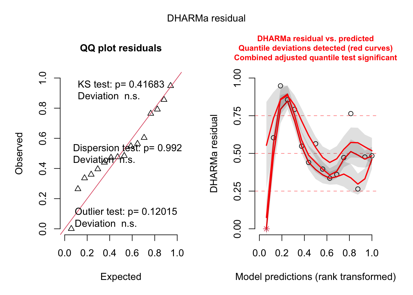
# diagnostics from DHARMa
DHARMa::simulateResiduals(model, plot = TRUE)

Object of Class DHARMa with simulated residuals based on 250 simulations with refit = FALSE . See ?DHARMa::simulateResiduals for help. 
 
Scaled residual values: 0.484 0.476 0.264 0.764 0.472 0.36 0.336 0.396 0.564 0.44 0.548 0.792 0.856 0.948 0.604 0

Code

# summary
summary(model)


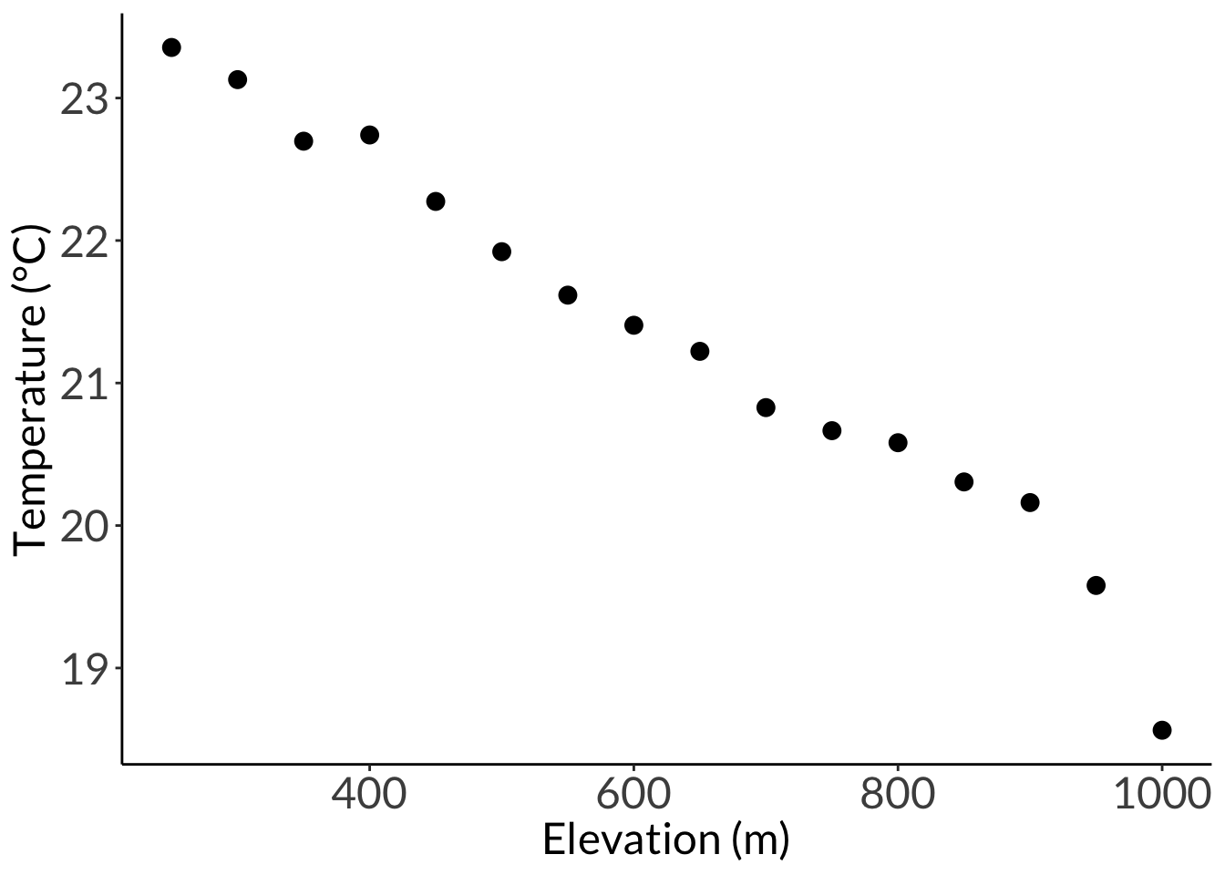
Call:
lm(formula = mean_temp_c ~ elevation_m, data = sonadora_sum)

Residuals:
     Min       1Q   Median       3Q      Max 
-0.67288 -0.07577  0.00022  0.09393  0.37042 

Coefficients:
              Estimate Std. Error t value Pr(>|t|)    
(Intercept) 24.7807991  0.1719438  144.12  < 2e-16 ***
elevation_m -0.0055446  0.0002581  -21.48 4.08e-12 ***
---
Signif. codes:  0 '***' 0.001 '**' 0.01 '*' 0.05 '.' 0.1 ' ' 1

Residual standard error: 0.238 on 14 degrees of freedom
Multiple R-squared:  0.9706,    Adjusted R-squared:  0.9684 
F-statistic: 461.4 on 1 and 14 DF,  p-value: 4.075e-12

Code

tidy(model)

# A tibble: 2 × 5
  term        estimate std.error statistic  p.value
  <chr>          <dbl>     <dbl>     <dbl>    <dbl>
1 (Intercept) 24.8      0.172        144.  1.32e-23
2 elevation_m -0.00554  0.000258     -21.5 4.08e-12

Code

# model predictions
ggpredict(model) |> plot(show_data = TRUE)

Code

# diagnostics
par(mfrow = c(2, 2))
plot(model)

6. correlation

a. abalone correlation

Code

cor.test(abalone_clean$ph, abalone_clean$change_in_area,
         method = "pearson")


    Pearson's product-moment correlation

data:  abalone_clean$ph and abalone_clean$change_in_area
t = 3.9265, df = 9, p-value = 0.003477
alternative hypothesis: true correlation is not equal to 0
95 percent confidence interval:
 0.3721101 0.9443471
sample estimates:
      cor 
0.7946121

b. correlation but different slopes

Code

corr_df <- tibble(
  x = seq(from = 1, to = 10, by = 0.5),
  y1 = 0.25*x,
  y2 = 1*x
) 

corr_0.25 <- ggplot(data = corr_df,
                    aes(x = x,
                        y = y1)) +
  geom_point(size = 3) +
  scale_y_continuous(limits = c(0, 10))

corr_1 <- ggplot(data = corr_df,
                 aes(x = x,
                     y = y2)) +
  geom_point(size = 3) +
  scale_y_continuous(limits = c(0, 10))

corr_0.25 + corr_1

c. no correlation but clear relationship

Code

x_lm <- seq(from = 1, to = 30, length.out = 50)
# y = a( x – h) 2 + k
df_para <- cbind(
  x = x_lm,
  y = 0.1*(x_lm - 15)^2 + 12
) |> 
  as_tibble()

ggplot(data = df_para, 
       aes(x = x, 
           y = y)) +
  geom_point(size = 3)

Code

cor.test(df_para$x, df_para$y, method = "pearson")


    Pearson's product-moment correlation

data:  df_para$x and df_para$y
t = 0.90749, df = 48, p-value = 0.3687
alternative hypothesis: true correlation is not equal to 0
95 percent confidence interval:
 -0.1540408  0.3939806
sample estimates:
      cor 
0.1298756

exponential growth example

Code

x_ex <- seq(from = 5, to = 9, length = 30)

y_ex <- exp(x_ex)

df_ex <- cbind(
  x = x_ex,
  y = -exp(x_ex)
) |> 
  as_tibble()

lm_ex <- lm(y ~ x, data = df_ex)

lm_ex


Call:
lm(formula = y ~ x, data = df_ex)

Coefficients:
(Intercept)            x  
       9431        -1642

model summary

Code

summary(lm_ex)


Call:
lm(formula = y ~ x, data = df_ex)

Residuals:
    Min      1Q  Median      3Q     Max 
-2756.1  -660.5   226.3   843.2  1081.0 

Coefficients:
            Estimate Std. Error t value Pr(>|t|)    
(Intercept)   9431.3     1111.3   8.486 3.16e-09 ***
x            -1642.0      156.5 -10.492 3.30e-11 ***
---
Signif. codes:  0 '***' 0.001 '**' 0.01 '*' 0.05 '.' 0.1 ' ' 1

Residual standard error: 1023 on 28 degrees of freedom
Multiple R-squared:  0.7972,    Adjusted R-squared:   0.79 
F-statistic: 110.1 on 1 and 28 DF,  p-value: 3.298e-11

model plots

Code

lm_pred <- ggpredict(lm_ex, terms = ~x)

ex_plot_noline <- ggplot(df_ex, aes(x= x, y = y)) +
  geom_point(shape = 17, size = 3, color = "orange") +
  theme_classic() +
  theme(text = element_text(size = 14))

ex_plot <- ggplot(df_ex, aes(x= x, y = y)) +
  geom_point(shape = 17, size = 3, color = "orange") +
  geom_line(data = lm_pred, aes(x = x, y = predicted), linewidth = 1) +
  theme_classic() +
  theme(text = element_text(size = 14))

diagnostic plots

Code

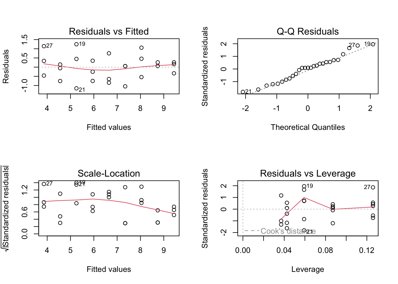
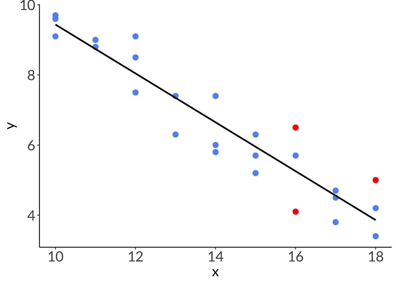
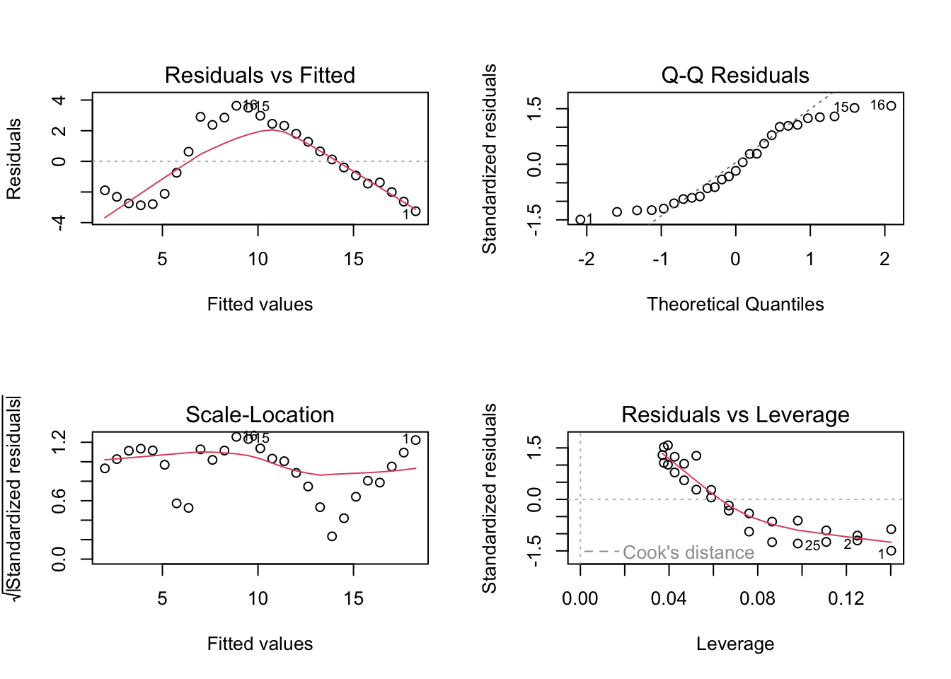
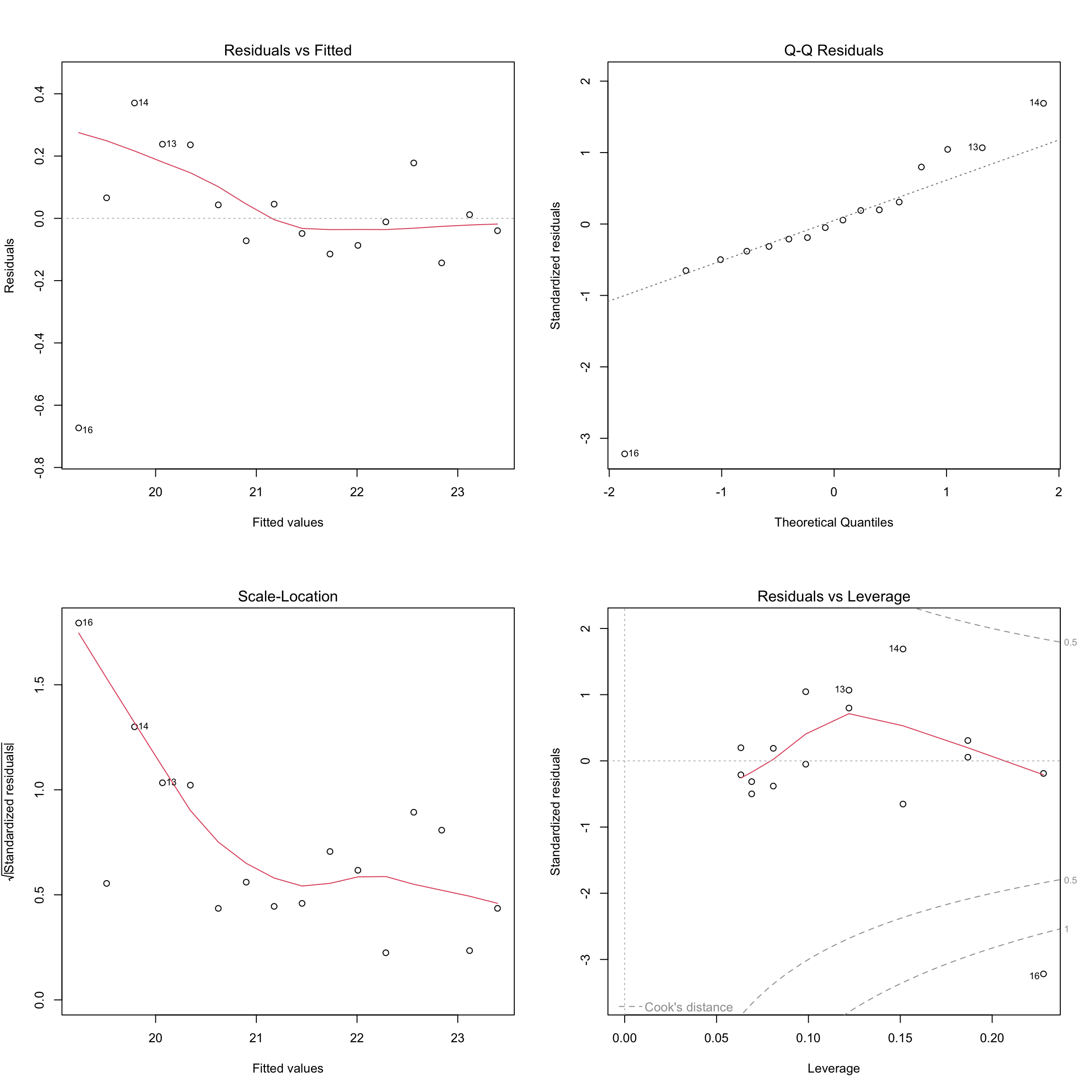
par(mfrow = c(2, 4))
plot(model1, which = c(1), col = "cornflowerblue", pch = 19)
plot(lm_ex, which = c(1), col = "orange", pch = 17)
plot(model1, which = c(2), col = "cornflowerblue", pch = 19)
plot(lm_ex, which = c(2), col = "orange", pch = 17)
plot(model1, which = c(3), col = "cornflowerblue", pch = 19)
plot(lm_ex, which = c(3), col = "orange", pch = 17)
plot(model1, which = c(5), col = "cornflowerblue", pch = 19)
plot(lm_ex, which = c(5), col = "orange", pch = 17)
dev.off()

Citation

BibTeX citation:

@online{bui2025,
  author = {Bui, An},
  title = {Week 7 Figures - {Lectures} 12 and 13},
  date = {2025-05-12},
  url = {https://spring-2025.envs-193ds.com/lecture/lecture_week-07.html},
  langid = {en}
}

For attribution, please cite this work as:

Bui, An. 2025. “Week 7 Figures - Lectures 12 and 13.” May 12, 2025. https://spring-2025.envs-193ds.com/lecture/lecture_week-07.html.