Due on Wednesday May 7 (Week 6) at 11:59 PM
Description
In this midterm, you will demonstrate your ability to synthesize lecture concepts and technical skills from workshop. At this point, you have the conceptual ideas you need (for example, what is the appropriate test to use if you want to compare groups?) and the technical skills you need (for example, summarizing data, visualizing data). You also have the investigative skills you need (for example, reading for tasks, googling!). You will use all these components to complete the midterm.
This midterm is open note, open internet, open everything; feel free to also talk with classmates and friends.
Set up tasks
As usual, create a new folder in your ENVS-193DS folder for midterm materials (a logical folder name would be midterm). Create an Rproject. Download all materials from Canvas into your midterm folder.
Start a new Quarto or RMarkdown document for your midterm. Make sure you read in your packages and data only at the top of the document.
Read in and store the data for Problem 3 as an object called tussocks.
Read in and store the data for Problem 4 as an object called rain.
Do we have a template?
You will not have a template.
You are responsible for creating a new Quarto document, setting the document up (i.e. reading in packages and data at the top of the doc), and making sure it renders properly (as a PDF or word doc, with the title, your name, and the date).
Stuck? See the video on Canvas about creating and rendering Quarto documents for help.
If you are using RMarkdown, the process is the same.
Problems
Problem 1. Understanding and critiquing written communication (20 points)
Skills you will demonstrate
In this problem, you will be responsible for demonstrating your understanding of the different components of a statistical test. All numbers describe a different statistical concept; how well do you understand what those numbers represent?
Description
You’re a fisheries manager interested in the effects of marine protected areas on the size of California sheephead (Bodianus pulcher). You find a study in which researchers examined exactly this effect. In their results section, the researchers wrote:
We found a difference in sheephead length (in centimeters) between marine protected areas and non-protected areas (Welch’s two-sample t-test, t(83.6) = 7.2, p < 0.001, \(\alpha\) = 0.05).
Components
a. Hypotheses (4 points)
The researchers didn’t state their hypotheses explicitly anywhere in their paper. In one sentence each, write the null (\(H_0\)) and alternative (\(H_A\)) hypotheses in statistical terms.
b. Test type (2 points)
The researchers ran a Welch’s two sample t-test. What must have been true for them to use a Welch’s t-test? Respond in 1 or 2 sentences only.
c. Test summary components (10 points)
In parentheses, the researchers cite some information about their statistical test:
t(105.6) = 6.6, p < 0.001, \(\alpha\) = 0.05
In one sentence each, explain the meaning of:
- t
- 105.6
- 6.6
- p < 0.001
- \(\alpha\) = 0.05
Be specific: what is the term that describes the component, and what does that component represent?
d. Missing information (4 points)
Unfortunately, this one sentence is the extent of the researchers’ communication about their statistics. Identify 2 other components or statistics they could have included (note that there may be more than 2 additional components that could make sense).
For each of your pieces of “missing information”, explain why it would be relevant to the questions or hypotheses.
Problem 2. Interpretation and communication (41 points)
Skills you will demonstrate
In this problem, you will be responsible for interpreting the results of a test with which you may be familiar, but haven’t seen. You will also demonstrate your ability to interpret code output and synthesize the statistics in writing to ground the stats in biology for a scientific audience.
Description
In 2014, the emergency manager of Flint, Michigan (mandated by the governor of Michigan at the time) switched the source of water for Flint from the Detroit River/Lake Huron to the Flint River. As a result, residents of Flint were exposed to lead contamination in their water. This was the start of the Flint water crisis, and Flint residents continue to deal with water contamination to this day.
When the crisis started, city officials recommended that residents allow pipes to clear (by flushing the pipes) before using any water. In 2015, Flint residents participated in a study to collect water samples to test for lead. Residents took water samples from their own taps at three different time points (letting the water run the whole time):
- immediately after turning on the water
- 45 seconds after turning on the water
- 2 minutes after turning on the water.
In this problem, you will work with statistical results from tests run on this data set of lead concentration in water samples collected by Flint residents. You will interpret statistical results to answer the questions:
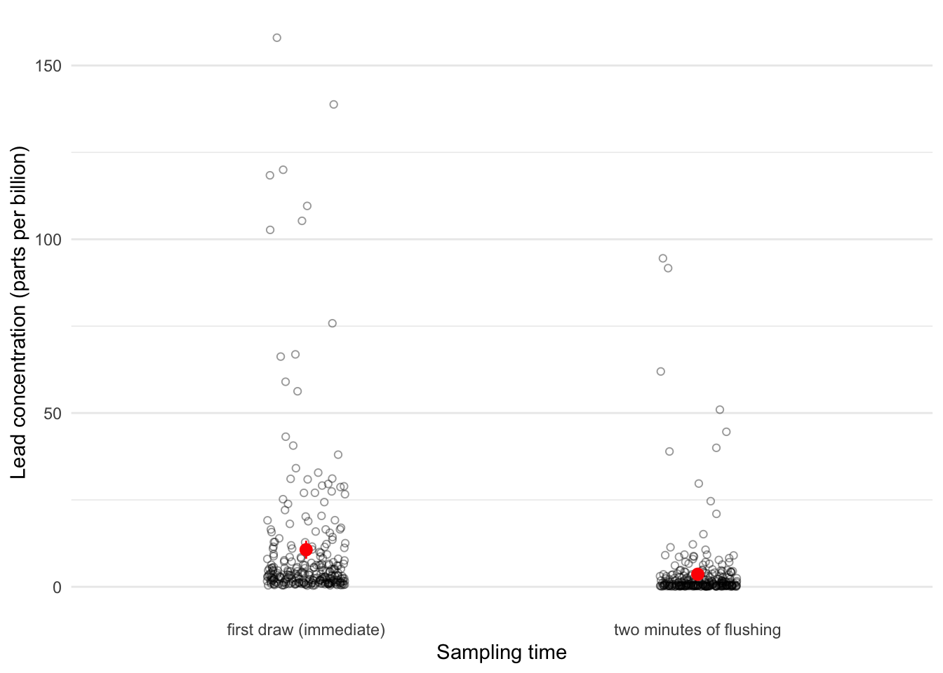
- Is there a difference in lead concentration (measured in parts per billion, ppb) between water samples taken immediately after turning on the water and 2 minutes after turning on the water?
- Is the amount of lead in the water after 2 minutes different from 0?
Before completing this problem, read about the study here. Additionally, make sure you understand the following figure:
Figure 1. Lead concentrations (ppb) in Flint, Michigan water samples. Water samples were taken from faucets immediately after turning the water on (“first draw (immediate)”) and 2 minutes after turning the water on (“two minutes of flushing”). Open circles represent a water sample taken from a single faucet (n = 300). Red points represent means and 95% confidence intervals. Data from Flint Water Study.
Components
a. Hypotheses (8 points)
In one sentence each, write your null (\(H_0\)) and alternative (\(H_A\)) hypotheses in statistical terms to answer the questions:
- Is there a difference in lead concentration (measured in parts per billion, ppb) between water samples taken immediately after turning on the water and 2 minutes after turning on the water?
- Is the amount of lead in the water after 2 minutes different from 0?
You should have one null and alternative for question 1, and one null and alternative for question 2.
b. Paired t-test (15 points)
This is the result of a paired t-test, which is appropriate when test subjects are measured twice in a paired study (in this case, water samples were taken at two time points from a single faucet). This would address question 1: Is there a difference in lead concentration (measured in parts per billion, ppb) between water samples taken immediately after turning on the water and 2 minutes after turning on the water?
    Paired t-test

data:  flint_clean$pb_bottle_1_ppb_first_draw and flint_clean$pb_bottle_3_ppb_2_mins_flushing
t = 6.3963, df = 268, p-value = 7.055e-10
alternative hypothesis: true mean difference is not equal to 0
95 percent confidence interval:
 4.881162 9.222377
sample estimates:
mean difference
        7.05177
This is the result of a calculation of effect size:
For paired samples, 'repeated_measures_d()' provides more options.Cohen's d | 95% CI
------------------------
0.39 | [0.27, 0.51]In 1-2 sentences only, summarize your interpretation and results of the test along with the effect size. Be sure to include all components of the test summary (for example, degrees of freedom, distribution, test statistic, confidence interval, etc.) that are important for understanding its structure.
Where necessary, round values to 1 decimal point and/or express as < 0.001.
c. One-sample t-test (15 points)
This is the output of a one-sample t-test to answer question 2: Is the amount of lead in the water after 2 minutes different from 0?
    One Sample t-test

data:  flint_clean$pb_bottle_3_ppb_2_mins_flushing
t = 5.6212, df = 268, p-value = 4.753e-08
alternative hypothesis: true mean is not equal to 0
95 percent confidence interval:
 2.347136 4.877629
sample estimates:
mean of x
 3.612383
In 1-2 sentences only, summarize your interpretation and results of the test. Be sure to include all components of the test summary (for example, degrees of freedom, distribution, test statistic, confidence interval, etc.) that are important for understanding its structure.
Where necessary, round values to 1 decimal point and/or express as < 0.001.
As stated by the Environmental Protection Agency (EPA), “EPA has set the maximum contaminant level goal for lead in drinking water at zero because lead is a toxic metal that can be harmful to human health even at low exposure levels” (EPA). In your response, contextualize these results within the EPA maximum contaminant goal (for example, are the samples from Flint on average more, less, or at the EPA maximum contaminant goal for lead?).
d. Statistical implications (5 points)
Imagine that you are a scientific advisor on water quality. Write 4-5 sentences about the results of both these tests in their real world context.
How would you communicate with the Flint residents who participated in this study about the results of both of these tests? Additionally, what do you make of these results within the context of the Flint water crisis, which is ongoing in 2025?
Data collection is always attached to its social context
The leader of this study was Dr. Marc Edwards of Virginia Tech, who claimed to represent the residents of Flint. After the original study was over, his group collected new samples from Flint residents and declared that the water was safe to use. However, residents knew the water was unsafe to use given lead and other contaminants, and filed a complaint against Dr. Edwards.
Problem 3. Reproducing an analysis (73 points)
Skills you will demonstrate
In environmental studies, open research means that researchers make their data and/or their code available for anyone to see. This means that anyone should be able to reproduce the analysis, even if they are not on the research team. In this problem, you will demonstrate your ability to read a paper to understand the context for a research study and its statistical analysis. You will then demonstrate your ability to take a data set and analyze it, using the researchers’ original analysis as a guide.
Description
You will reproduce the analysis in: Steketee, Jess K., Adrian V. Rocha, Laura Gough, Kevin L. Griffin, Ian Klupar, Ruby An, Nicole Williamson, and Rebecca J. Rowe. 2022. “Small Herbivores with Big Impacts: Tundra Voles (Microtus Oeconomus) Alter Post-Fire Ecosystem Dynamics.” Ecology 103(7): e3689. https://doi.org/10.1002/ecy.3689
Read all parts of the paper before starting this problem.
You will specifically recreate the components in this passage:
Although tussock density was lower at the burned site, tussocks were larger.
Getting the data
This statement relies on the dataset stored here:
Rocha, A. 2021. Tussock height and diameter in moist acidic tussock tundra at the site of the 2007 Anaktuvuk River fire scar, and nearby unburned tundra measured in 2016 ver 1. Environmental Data Initiative. https://doi.org/10.6073/pasta/1dccd3fdb3aa693f9c2b69a24f8306ed
Download the data into your midterm directory. To understand the data structure, read the metadata (under Resources > View full metadata > Data Entities).
Components
a. Variables (4 points)
In 1-2 sentences, describe the response variable (with units) and predictor variable (include each group). Be sure to explain the type of each variable (categorical, continuous, etc.).
b. Hypotheses (4 points)
In one sentence each, write the null (\(H_0\)) and alternative (\(H_A\)) hypotheses in statistical terms.
c. Cleaning and organizing data (10 points)
Response variable column in original dataset
Use the “Average Moss (cm)” column for tussock height.
Create an object called tussocks_clean. Clean the data by:
cleaning all the column names
replacing the values in the
sitecolumn as follows:- replace
SevwithBurned
- replace
UnbwithUnburned
- replace
selecting only the site and height column
Use the pipe operator to string functions together.
Once you are done, display 5 rows from tussocks_clean using the slice_sample() function. DO NOT SUBSET THE DATA FRAME. THIS IS FOR DISPLAYING THE CONTENTS ONLY.
d. Summarizing and table displays (12 points)
Create an object called tussocks_summary using the tussocks_clean data frame to calculate the:
- means,
- standard deviations,
- standard errors, and
- 95% confidence intervals of the means
for the response variable within the two groups.
Round all numbers to 1 decimal point.
Display only the means, standard deviations, standard errors, and 95% confidence intervals in a table. Choose one of the following packages to do so:
Make sure the column names of the table are polished (no underscores, capitalized in sentence case).
Show all code for your calculations and making/polishing the table.
Double check your table!
Render your document to make sure your table looks right. Do not assume that just because your code works, your table will render correctly.
e. Tests and effect sizes (6 points)
Use a Welch’s t-test to compare mean tussock height between groups.
Calculate the appropriate effect size.
f. Written communication (15 points)
The authors communicated about the results of this test in the text above (in the Description) and in a table in the paper.
In 1-2 sentences only, write an updated interpretation with results of the test and effect size. Be sure to include all components of the test summary (for example, degrees of freedom, distribution, test statistic, confidence interval, etc.) that are important for understanding its structure.
g. Making a new figure (13 points)
Plots like Figure 3b in the paper show means and whiskers (in this case, standard error), but do not show the data structure and can mask important information about the spread of the observations in each sample.
Make a new figure that displays the mean and standard error (as in figure 3b) but shows the underlying data. For full credit:
- take out the gridlines and make the plot and panel background white
- jitter the observations horizontally but not vertically
- give each type a different color that is different from the
ggplot()default color
- use transparent open circles to represent the underlying data
- take out the legend
- include a plot title and put your name as the subtitle
h. Caption (10 points)
Write a caption for your figure in part g. Include a data citation.
Problem 4. Cleaning, wrangling, and visualization (33 points)
Skills you will demonstrate
Figures are built on data; however, to make a figure, you need to understand the data structure and any cleaning, wrangling, or summarizing steps to create it. In this problem, you will demonstrate your ability to clean, wrangle, and/or summarize a data set to create a figure, using a final figure as a guide.
Description
In this problem, you will use a data set of rainfall (measured in inches) from the rain gauge on top of Ellison Hall to recreate this figure.
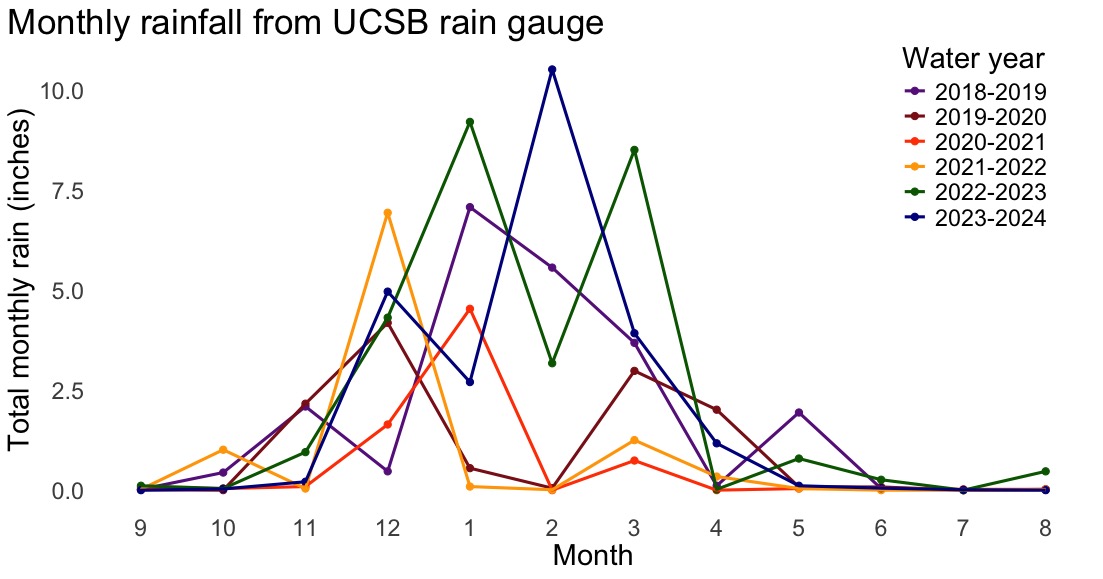
The caption for the figure is as follows:
Figure 2. Most rain occurs between November and March. Lines and points represent total monthly rain (measured in inches) from Ellison Hall rain gauge for each water year starting in September and ending in August. Shown are water years 2018-2019 (purple), 2019-2020 (red), 2020-2021 (orange), 2021-2022 (yellow), 2022-2023 (green) and 2023-2024 (blue). Data source: County of Santa Barbara Public Works, Daily Rainfall Data (XLS). Accessed April 2025.
Getting the data
This data set comes from the Count of Santa Barbara Public Works under the Daily Rainfall Data (XLS) page.
On the website, click the red dot next to Isla Vista (this represents the Ellison Hall rain gauge).
MAKE SURE YOU HAVE DOWNLOADED THE CORRECT DATA FILE. YOUR FILE SHOULD BE CALLED 200dailys.xls.
Look at the data in Sheets or Excel before starting!
You will see that there is extra information at the top of the sheet. Clean up the file so that it only has data columns, and save that as a .csv file.
Components
a. Initial cleaning, wrangling, and summarizing (14 points)
Double check your data
Before you do this problem, make sure you have code to read in and save your data as an object called rain at the top of the document.
The following chunk of code creates an object called rain_clean. Copy and paste this code into your document to run it.
Where prompted in the code annotations, fill in your responses to describe what each function is doing, and how the data frame changes. Only write your responses in the annotations. See function 7 for an example.
rain_clean <- rain |>

  # 1. what changes after this function?
  # [insert response here]
  # give an example.
  # [insert response here]
  clean_names() |>

  # 2. what new column is created?
  # [insert response here]
  # give an example of a value in this column.
  # [insert response here]
  mutate(water_year_minus1 = water_year - 1) |>

  # 3. what old column is changed?
  # [insert response here]
  # give an example of a value in the old column, and explain how it changed.
  # [insert response here]
  mutate(water_year = paste0(water_year_minus1, "-", water_year)) |>

  # 4. what columns are excluded from the data frame?
  # [insert response here]
  # give an example of a value in water_year_minus1
  # [insert response here]
  # give an example of a value in code
  # [insert response here]
  select(!c(water_year_minus1, code)) |>

  # 5. which column is manipulated, and what changes about it?
  # Hint: run str(rain_clean) in the Console. what do you see for the month column?
  # [insert response here]
  mutate(month = as_factor(month),
         month = fct_relevel(
           month,
           "9", "10", "11", "12", "1", "2", "3", "4", "5", "6", "7", "8")
         ) |>

  # 6. what is being calculated? on an annual, monthly, or daily scale?
  # [insert response here]
  # give an example.
  # [insert response here]
  group_by(month, water_year) %>%
  summarize(total_rain = sum(daily_rain, na.rm = TRUE)) |>
  ungroup() |>

  # 7. what is being done to which columns?
  # missing combinations of values of water_year and month are being filled in with 0
  # give an example.
  # july in 1951-1952 was not in the data frame previously, and now is present with a total rain of 0 inches
  complete(water_year,
           month,
           fill = list(total_rain = 0)) |>

  # 8. which observations are kept after this filtering step?
  # [insert response here]
  filter(water_year %in% c("2018-2019",
                           "2019-2020",
                           "2020-2021",
                           "2021-2022",
                           "2022-2023",
                           "2023-2024"))
A possible approach
One way to approach this problem is to delete all the pipe operators and add them back in one by one. With every additional function, look at the rain_clean object to describe what has changed about the data frame.
b. Make the figure (19 points)
Recreate the figure. Specifically, recreate the:
- x-axis (and label),
- y-axis (and label),
- title,
- legend position,
- panel background (blank),
- axis lines and ticks (blank),
- title position,
- geometries, and
- different colors
Note that you do not need an exact match of the colors (choose whatever colors you want) or legend position (just make sure it’s inside the panel and doesn’t cover any points).
My figure doesn’t look right when I render my document.
You will have to set the code chunk options to make a larger figure. Click the gear button in the code chunk to set those options.
Checklist
Your submission should:
Additionally, your submission should only include the components listed below:
for Problem 1:
for Problem 2:
for Problem 3:
for Problem 4:
Lastly, check out the rubric on Canvas to see the point breakdown in more detail.
200 points total